anomaly documentation
The anomaly function plots line data with different colors of shading filling the area between the curve and a reference value. This is a common way of displaying anomaly time series such as sea surface temperatures or climate indices.
Back to Climate Data Tools Contents
Contents
Syntax
anomaly(x,y)
anomaly(...,'thresh',thresholdValue)
anomaly(...,'top',ColorSpec)
anomaly(...,'bottom',ColorSpec)
anomaly(...,'LineProperty',LineValue)
[hlin,htop,hbot] = anomaly(...)
Description
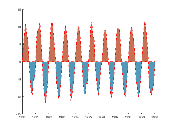
anomaly(x,y) plots a black line with red filling the area between zero and line any line values above zero; blue fills the area between zero and any values below zero.
anomaly(...,'thresh',thresholdValue) specifies the value(s) beyond which are shaded. By default the threshold value is zero, meaning everything above or below zero is shaded. If shading is desired relative to some value other than zero, specify that value as a scalar threshold. If shading is desired only below some lower threshold and above an upper threshold, specify the thresholdValue as a two element array (e.g., let thresholdValue be [-0.4 0.5] to shade all values less than -0.4 or greater than 0.5).
anomaly(...,'topcolor',ColorSpec) specifies the top color shading, which can be described by RGB values or any of the Matlab short-hand color names (e.g., 'r' or 'red').
anomaly(...,'bottomcolor',ColorSpec) specifies the bottom shading color.
anomaly(...,'LineProperty',LineValue) sets any line properties such as 'color' or 'linewidth'.
[hlin,htop,hbot] = anomaly(...) returns the graphics handles of the line, top, and bottom plots, respectively.
Example 1: Simple
Plot this sample data:
x = 1990:1/12:2000;
y = 10*sin(2*pi*x) + randn(size(x));

anomaly(x,y)

Example 2: Specify shading colors and line properties
Using the same x and y data as above, make the line thick, red, and dashed:
figure
anomaly(x,y,'color','r','linewidth',2,'linestyle','--')
Or have no line at all, while making the top seafoam blue and the bottom sort of orangish. Use the rgb function to get the RGB values of such colloquial color names:
figure
anomaly(x,y,'color','none','top',rgb('seafoam blue'),...
   'bottom',rgb('orangish'))

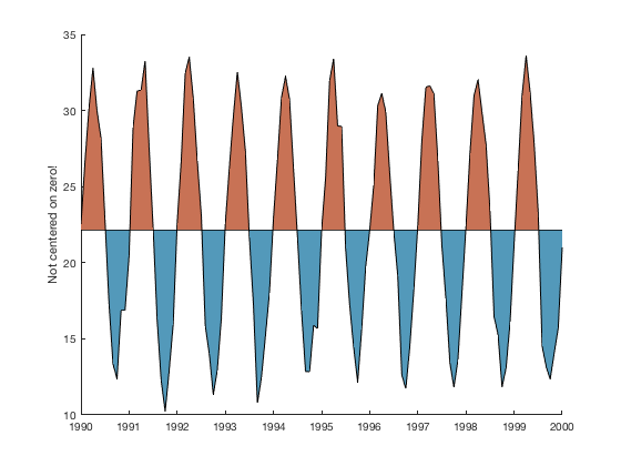
Example 3: Anomalies about a nonzero value
Sometimes anomalies are not relative to zero, but are relative to their mean. Perhaps you have some temperature values that fluctuate around 22 degrees:
figure

anomaly(x,y+22,'thresh',mean(y+22))

ylabel 'Not centered on zero!'
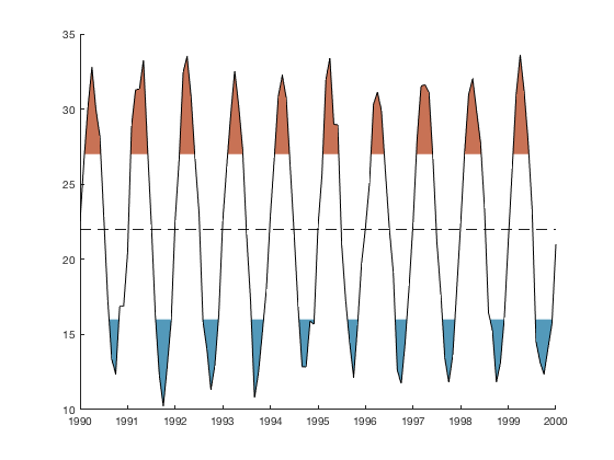
Example 4: Thresholding
Only shade in the regions less than 16 or greater than 27. Use hline to add a horizontal black line at the y value of 22 if you desire:
figure

anomaly(x,y+22,'thresh',[16 27])

hline(22,'k--') % places a horizontal line at y=22.
Author Info
This function was written by Chad A. Greene of the University of Texas Institute for Geophysics (UTIG), January 2017.