`cube2rect` documentation

The cube2rect function reshapes a 3D matrix for use with standard Matlab functions.

cube2rect enables easy, efficient, vectorized analysis instead of using nested loops to operate on each row and column of a matrix. Its complement is rect2cube.

Back to Climate Data Tools Contents

Syntax
Description
Why does this function exist?
Example 1a: A simple 2x2 grid
Example 1b: Masking regions of data
Example 2: Sea surface temperatures:
Author Info

Syntax

A2 = cube2rect(A3)
A2 = cube2rect(A3,mask)

Description

A2 = cube2rect(A3) for a 3D matrix A3 whose dimension correspond to space x space x time, cube2rect reshapes the A3 into a 2D matrix A2 whose dimensions correspond to time x space.

A2 = cube2rect(A3,mask) uses only the grid cells corresponding to true values in a 2D mask. This option can reduce memory requirements for large datasets where some regions (perhaps all land or all ocean grid cells) can be neglected in processing.

Why does this function exist?

Good question! The short answer is it enables fast and easy vectorization, meaning no more nested loops. A more nuanced explanation with lots of examples can be found in this Tutorial on 3D data analysis.

Example 1a: A simple 2x2 grid

Consider this 2x2 grid. At time 1, values are just over 100. By time 2, all of the values have increased by 100, except the lower left grid cell that increases by 120. And the trend continues at time 3, where all the values are on the order of 300. Here's the data:

% First time slice:
A(:,:,1) = [101 103;
            102 104];

% Second time slice:
A(:,:,2) = [201 203;
            222 204];

% Third time slice:
A(:,:,3) = [301 303;
            342 304];

Many standard Matlab functions operate down columns of 2D matrices, and we can easily use those functions if we reshape A such that one dimension corresponds to time and the other dimension corresponds to space. Here's how to reshape A with cube2rect:

cube2rect(A)

ans =
   101   102   103   104
   201   222   203   204
   301   342   303   304

Now each column corresponds to a grid cell in A and each row corresponds to time. It's like this:

    s p a c e
   ---------->
t | 101   102   103   104
i | 201   222   203   204
m | 301   342   303   304
e v

Example 1b: Masking regions of data

If you want to perform computationally intensive operations on a large dataset, it can sometimes help to mask out all the grid cells that don't need to be analyzied. For example, if you have a high resolution global dataset with lots of measurements through time, you might want to use island to mask out land areas or ocean areas, and only peform analysis on the regions of interest. Using the simple 2x2 dataset from above, here's what it would look like if you want to mask out the upper right grid cell before reshaping A:

mask = [true false;
        true true]

cube2rect(A,mask)

mask =
  2×2 logical array
   1   0
   1   1
ans =
   101   102   104
   201   222   204
   301   342   304

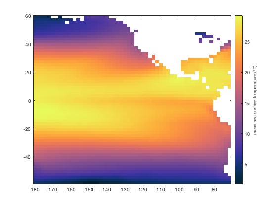
Example 2: Sea surface temperatures:

Fake data can feel a bit abstract, so let's look at how you might employ cube2rect with real climate data.

load pacific_sst

In the pacific_sst sample dataset, we have an sst variable with the dimensions

size(sst)

ans =
    60    55   802

which corresponds to 60 latitude grid cells, 55 longitude grid cells, and 802 monthly solutions. To calculate the mean sea surface temperature at each grid cell, we could specify the third dimension of sst when calling mean like this:

meanSST = mean(sst,3);

imagescn(lon,lat,meanSST)
cmocean thermal
cb = colorbar;
ylabel(cb,'mean sea surface temperature (\circC)')

Yeah, of course you can get the mean sea surface temperature that easy, but cube2rect is intended to allow more applications than just the built in mean, std, etc. So let's use cube2rect to get get a plot of the mean SST, just like the one above. First, reshape the 3D sst matrix:

sstr = cube2rect(sst);

size(sstr)

ans =
         802        3300

Now the reshaped sstr matrix contains 802 rows corresponding to each of the 802 time steps, and 3300 columns which correspond to each of the 60x55 grid cells. Calculating the mean sea surface temperature at each grid cell is easy now:

my_meanSST_2d = mean(sstr);

size(my_meanSST_2d)

ans =
           1        3300

Now my_meanSST contains just one row--that's a single mean value for each of the 3300 grid cells. To get those grid cells back into their original shape, use rect2cube. It's the yin to cube2rect's yang.

my_meanSST_3d = rect2cube(my_meanSST_2d,[60 55 802]);

imagescn(lon,lat,my_meanSST_3d)
cmocean thermal
cb = colorbar;
ylabel(cb,'mean sea surface temperature')

Author Info

This function and supporting documentation were written by Chad A. Greene of the University of Texas Institute for Geophysics (UTIG).

cube2rect documentation

Contents